Generic 9: Density scaling of infectivity

This tutorial explores the effect of population density on the transmissibility of disease.

By default, the EMOD executable (Eradication.exe) uses frequency-dependent transmission and the overall transmissibility does not change with population size or density. An infected individual will infect the same number of people either in a small village or in a metropolitan area. However, it is possible when population size is low, the transmissibility might be less and follow density- dependent behavior instead of frequency-dependent behavior.

Based on existing evidence, it is possible that neither a frequency-dependent nor a density- dependent mechanism may adequately describe the correct scaling over the entire population density spectrum. The EMOD executable uses the spatial contact model with constant population density and limited activity range to estimate contact rates as discussed in the article The scaling of contact rates with population density for the infectious disease models, by Hu et al., 2013 Journal of Mathematical Bioscience. 244(2):125-134. The scaling function can be specified for β, in the form of:

β = β₀ (1- e ρ/ρ_c50)

where ρ_c50 is a constant determining the speed of increase of infectivity.

For this tutorial, the simulation is run three times with a different node size for each run. The change of node grid size will result in the change of population density for the simulations.

Demographics inputs

This tutorial uses generic_scenarios_demographics file for demographics input. You can view the complete demographics file at <path_to_directory>RegressionScenariosInputFiles where <path_to_directory> is the location where EMOD source files were installed. For more information on demographics files, see Demographics parameters.

Key configuration parameters

The tutorial simulates the person-person disease transmission of an influenza-like-illness model with waning immunity (SEIRS) over a short period, in a hypothetical community over a short period. After infection, all individuals will stay immune for a certain period of time before they become susceptible again. The saturated R₀is set to 1.5 and R₀initially increases with population density

You can view the complete config.json at <path_to_directory>RegressionScenariosGeneric Scenarios09_DensityScaling directory.

SEIRS model setup parameters

The incubation period, infection period, immunity, and immunity waning, must be enabled for an SEIRS model. For more information, see Incubation and Immunity parameters.

Set the following parameters:

• Set Base_Incubation_Period to 3.
• Set Incubation_Period_Distribution to “FIXED_DURATION.”
• Set Enable_Immunity to 1.
• Set Enable_Immune_Decay to 1.

Disease parameters

These parameters set Eradication.exe to run an SEIRS-like disease model with person-to-person direct transmission. For more information, see Infectivity and transmission parameters.

Set the following parameters:

• Set Base_Infectivity to 0.375.
• Set Base_Infectious_Period to 14.
• Set Infectious_Period_Distribution to “FIXED_DURATION.”

Immunity parameters

The following parameters configure a 90 day immunity. After 90 days, the immunity is lost immediately. For more information, see Immunity parameters.

Set the following parameters:

• Set Acquisition_Blocking_Immunity_Duration_Before_Decay to 90.
• Set Transmission_Blocking_Immunity_Duration_Before_Decay to 90.
• Set Acquisition_Blocking_Immunity_Decay_Rate to 1.
• Set Transmission_Blocking_Immunity_Decay_Rate to 1.

Density scaling parameters

These parameters are used by the scaling function to calculate β. You can change Node_Grid_Size to change population density for different simulations. For more information, see Infectivity and transmission and Simulation setup parameters.

Set the following parameters:

• Set Population_Density_Infectivity_Correction to “SATURATING_FUNCTION_OF_DENSITY.”
• Set Population_Density_C50 to 30.
• Set Node_Grid_Size to 0.1, 0.15, and 0.3 respectively for the three different simulations.

Interventions

This simulation uses an OutbreakIndividual event for repeated infection seeding. The campaign.json file is in the ScenariosGeneric09_DensityScaling directory. For more information, see OutbreakIndividual parameters.

{
    "Use_Defaults": 1,
    "Events": [{
        "Campaign_Name": "Infections",
        "Event_Coordinator_Config": {
            "Coverage": 0.001,
            "Demographic_Coverage": 0.001,
            "Intervention_Config": {
                "Antigen": 0,
                "Event_Name": "Outbreak",
                "Genome": 0,
                "Outbreak_Source": "ImportCases",
                "class": "OutbreakIndividual"
            },
            "Number_Repetitions": 10,
            "Target_Age_Max": 100,
            "Target_Age_Min": 0,
            "Target_Demographic": "Everyone",
            "Timesteps_Between_Repetitions": 120,
            "class": "StandardInterventionDistributionEventCoordinator"
        },
        "Nodeset_Config": {
            "class": "NodeSetAll"
        },
        "Start_Day": 0,
        "class": "CampaignEvent"

    }]
}

Run the simulation

Run the simulation and generate graphs of the simulation output. For more information, see Run simulations.

Note

Because the EMOD model is stochastic, your graphs may appear slightly different from those given below.

Simulation output graphs

The simulation was run three times with the Node_Grid_Size set to three different values: 0.1, 0.15, and 0.3 degrees. The node was assumed to be near the equator (both latitude and longitude were set to 0) and the population was 10,000. Using the three different Node_Grid_Size values, the node area for the three simulations were 124, 278, and 1112 km² , respectively. With a population of 10,000, the population density was 80, 36, and 9 people/km², respectively.

Using the data described in the previous paragraph, the three densities correspond to different R:sub:0values: close to 1.5, close to 1, and well below 1, respectively, as shown in the following graph from Hu *et al*., 2013. *Journal of Mathematical Bioscience*. 244(2):125-134..

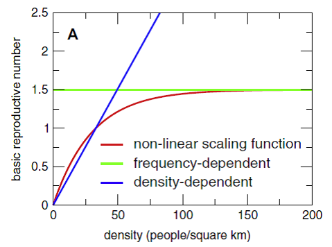
Figure 1: Effect of population density on transmissibility

The following table shows the values for the three simulations:

Simulation	Population	Latitude, Longitude	Node_Grid_Size	Node Area	Density	R0
1	10,000	0, 0	0.1	124	80	R0> 1
2	10,000	0, 0	0.15	278	36	R0~ 1
3	10,000	0, 0	0.3	1112	9	R0< 1

The following graphs show the effect of population density on transmissibility, in terms of maintaining endemic status. When population density is large enough, it is easy to maintain an endemic status while in lower density is difficult to do so.

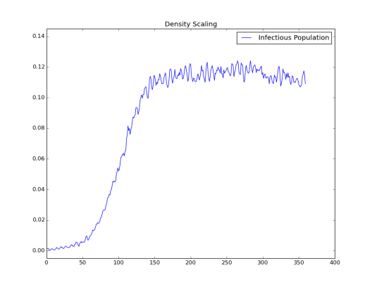
Simulation 1: Node_Grid_Size = 0.1, population density 80/km²and R₀ > 1

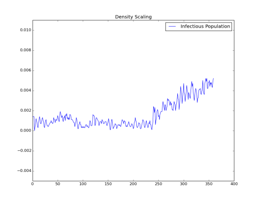
Simulation 2: Node_Grid_Size = 0.15, population density 36/km²and R₀ ~ 1

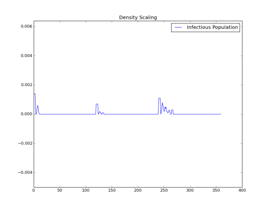
Simulation 3: Node_Grid_Size = 0.3, population density 9/km²and R₀ < 1

Exploring the model

Change the Node_Grid_Size to other values. Explore a range of population densities and run the simulation multiple times to get a probability of fade-out under different densities.

You can download the sample Excel file, calculate_cell_area_pop_density, to calculate the node area (cell area) and population density. There are four inputs that you can modify: latitude, longitude, grid size (in degrees) and population.

Click calculate_cell_area_pop_density to download the file.