The results structure
Charles Eliot
2023-09-22
results-struct.RmdThe script for a typical run of the PACE-HRH modeling engine looks like this:
library(pacehrh)

pacehrh::InitializePopulation()
pacehrh::InitializeScenarios()
pacehrh::InitializeStochasticParameters()
pacehrh::InitializeSeasonality()
pacehrh::InitializeCadreRoles()

scenario <- "MergedModel"

pacehrh::SetGlobalStartEndYears(2020, 2040)

results <-
  pacehrh::RunExperiments(scenarioName = scenario,
                       trials = 10)
In this note we describe the contents of the results data
structure returned by RunExperiments().
Structure
The results (plural) structure is an R list consisting of multiple result (singular) structures, one per trial.
length(results)
## [1] 10
Each result structure consists of the following parts:
- AnnualTimes
- AnnualCounts
- SeasonalityResults
- Population
- PopulationRates
names(results[[10]])
## [1] "AnnualTimes"        "AnnualCounts"       "SeasonalityResults"
## [4] "Config"             "Population"         "PopulationRates"
Overview of the calculations
The PACE-HRH modeling engine computes the total amount of time required to perform healthcare tasks, based on population predictions.
- Step 1: Build population predictions for a range of years, based on shifting mortality and fertility rates.
- Step 2: For each combination of healthcare task and year, use information about the task - applicable population group, disease prevalence, time required per task event, number of events, etc - to determine the number of times a task is performed per year (“services”), and the total amount of time required for all services in a given year.
- Step 3: Apply data about the per-month seasonality of healthcare events to convert the annual data into per-month data. This calculation happens in two phases. In the first phase a seasonality curve is applied to the annual data, distributing the annual value according to the seasonality curve across the twelve months of the year. In the second phase, offset data is used to place events in the actual months they occur. An example of this is ante-natal care: a future birth generates ante-natal care tasks 1, 3, 5, and 7 months before the birth happens.
For each trial in a suite of trials, the parameters that feed the calculations are varied stochastically to generate confidence interval predictions.
AnnualTimes
AnnualTimes holds the results of the time-per-task-per-year values (in minutes) calculated in Step 2. The results are in the form of a matrix, with tasks along the row dimension and years along the columns.
dim(results[[10]]$AnnualTimes)
## [1] 122  22
rownames(results[[10]]$AnnualTimes)
##   [1] "FH.MN.ANC.1"    "FH.MN.PNC.7"    "FH.MN.S.12"     "FH.MN.S.13"
##   [5] "FH.MN.S.14"     "FH.MN.15"       "FH.MN.17"       "FH.MN.18"
##   [9] "FH.MN.19A"      "FH.MN.19B"      "FH.MN.19C"      "FH.MN.19D"
##  [13] "FH.MN.23"       "FH.MN.24"       "FH.MN.29"       "FH.MN.30"
##  [17] "FH.EPI.31"      "FH.EPI.32A"     "FH.EPI.32B"     "FH.EPI.32C"
##  [21] "FH.EPI.32D"     "FH.EPI.33"      "FH.EPI.34"      "FH.EPI.35"
##  [25] "FH.EPI.36"      "FH.EPI.37"      "FH.FP.38A"      "FH.FP.38B"
##  [29] "FH.FP.38C"      "FH.FP.39"       "FH.FP.42"       "FH.FP.44"
##  [33] "FH.FP.45"       "FH.FP.47"       "FH.FP.48"       "FH.FP.49"
##  [37] "FH.FP.50"       "FH.FP.51"       "FH.FP.52"       "FH.FP.53"
##  [41] "FH.FP.58"       "FH.FP.59"       "FH.FP.62"       "FH.Ntr.64"
##  [45] "FH.Ntr.65"      "FH.Ntr.66"      "FH.Ntr.67"      "FH.Ntr.70"
##  [49] "FH.Ntr.71"      "FH.Ntr.74"      "FH.Ntr.75"      "FH.Ntr.76"
##  [53] "FH.Ntr.77"      "FH.Ntr.78"      "FH.Ntr.79"      "FH.Ntr.80"
##  [57] "FH.Ntr.81"      "FH.Ntr.82"      "FH.Ntr.83"      "FH.Ntr.84"
##  [61] "FH.Ntr.85"      "FH.Ntr.86"      "DPC.STI.95"     "DPC.STI.99"
##  [65] "DPC.Mlr.102"    "DPC.Mlr.105"    "DPC.Mlr.106"    "DPC.Mlr.107"
##  [69] "DPC.TB.108A"    "DPC.TB.108B"    "DPC.TB.110"     "DPC.Drug.112"
##  [73] "DPC.Drug.113"   "DPC.Drug.114"   "DPC.Cncr.115"   "DPC.Cncr.117"
##  [77] "DPC.Cncr.119A"  "DPC.Cncr.119B"  "DPC.Cncr.119C"  "DPC.Cncr.119D"
##  [81] "DPC.Cncr.119E"  "DPC.Cncr.119F"  "DPC.Cncr.119G"  "DPC.Cncr.119H"
##  [85] "DPC.Cncr.119I"  "DPC.Cncr.119J"  "DPC.Cncr.119K"  "DPC.Hyp.120"
##  [89] "DPC.Dbt.123"    "DPC.Asth.126"   "DPC.Asth.127"   "DPC.MH.130A"
##  [93] "DPC.MH.130B"    "DPC.MH.130C"    "DPC.MH.130D"    "DPC.MH.130E"
##  [97] "DPC.MH.130F"    "DPC.MH.131"     "DPC.MH.132"     "DPC.MH.133"
## [101] "DPC.MH.134"     "DPC.MH.135"     "DPC.Oph.136"    "DPC.Oph.137"
## [105] "DPC.Oph.140"    "DPC.NTD.156"    "DPC.NTD.157"    "DPC.NTD.159"
## [109] "DPC.NTD.160"    "DPC.NTD.162"    "DPC.NTD.163"    "DPC.NTD.164"
## [113] "DPC.NTD.168"    "DPC.NTD.169"    "DPC.NTD.171"    "DPC.NTD.172"
## [117] "DPC.NTD.175"    "MHH_HEH"        "MHH_HEP"        "Record keeping"
## [121] "Travel_HEH"     "Travel_HEP"
colnames(results[[10]]$AnnualTimes)
##  [1] "2020" "2021" "2022" "2023" "2024" "2025" "2026" "2027" "2028" "2029"
## [11] "2030" "2031" "2032" "2033" "2034" "2035" "2036" "2037" "2038" "2039"
## [21] "2040" "2041"
results[[10]]$AnnualTimes["FH.MN.ANC.1",]
##     2020     2021     2022     2023     2024     2025     2026     2027
## 5630.707 5594.612 5630.707 6099.932 5955.555 6099.932 6244.309 6172.121
##     2028     2029     2030     2031     2032     2033     2034     2035
## 6605.252 6894.006 6280.404 6605.252 7146.666 7363.232 7507.609 7940.740
##     2036     2037     2038     2039     2040     2041
## 8301.683 8157.306 8770.909 9059.663 9023.568 9204.040
AnnualCounts
AnnualCounts reports the number of times per year a healthcare task is performed.
results[[10]]$AnnualCounts["FH.MN.ANC.1",]
## 2020 2021 2022 2023 2024 2025 2026 2027 2028 2029 2030 2031 2032 2033 2034 2035
##  624  620  624  676  660  676  692  684  732  764  696  732  792  816  832  880
## 2036 2037 2038 2039 2040 2041
##  920  904  972 1004 1000 1020
# The pacehrh:::EXP environment holds working variables from the most recent trial.
# It's accessed here to illustrate how task time calculation are done.
print(pacehrh:::EXP$taskParameters["FH.MN.ANC.1",])
cat("\n")
print(pacehrh:::EXP$demographics[["2020"]]$Female + pacehrh:::EXP$demographics[["2020"]]$Male)
##  StartingRateInPop     RateMultiplier   AnnualDeltaRatio NumContactsPerUnit
##           1.000000           1.000000           1.000000           4.000000
##  NumContactsAnnual     MinsPerContact       HoursPerWeek
##           0.000000           9.023568           0.000000
##
##   [1] 156 150 144 140 138 136 134 133 131 128 126 123 121 119 117 115 115 113
##  [19] 111 109 107 105 103  99  95  93  89  85  80  76  72  68  66  63  60  59
##  [37]  57  55  53  50  47  45  43  42  40  38  37  36  34  32  31  30  28  27
##  [55]  25  24  23  21  21  20  19  19  18  17  17  15  15  13  13  13  11  11
##  [73]  11   9   9   8   7   6   6   5   4   4   3   2   2   2   2   2   1   0
##  [91]   0   0   0   0   0   0   0   0   0   0   0
In this example (ante-natal task FH.MN.ANC.1), there are 156 births in 2020 in a total population of 5000, each of which generates 4 ante-natal care visits (NumContactsPerUnit), giving 624 total visits. Each visit is 9.0235684 minutes long, a value derived from a stochastic variation of the base value of 10, to give a total time of 5630.7067108 minutes.
SeasonalityResults
As described above, the system takes the annual times reported in AnnualTimes, applies a seasonality curve to distribute the annual times across the months of the year, then uses seasonality offsets to place the healthcare events in the correct months.
Sample calculation
The FH.MN.ANC.1 task uses the Births seasonality curve, and has four offsets representing ante-natal care visits 1, 3, 5 and 7 months before a birth.
pacehrh:::BVE$seasonalityOffsets[pacehrh:::BVE$seasonalityOffsets$Task == "FH.MN.ANC.1",]
## # A tibble: 1 × 9
##   Task        Description Curve  Offset1 Offset2 Offset3 Offset4 Offset5 Offset6
##   <chr>       <chr>       <chr>    <dbl>   <dbl>   <dbl>   <dbl>   <dbl>   <dbl>
## 1 FH.MN.ANC.1 ANC visits  Births      -7      -5      -3      -1      NA      NA
The Births seasonality curve represents a normalized distribution (sum = 1) of the annual task time across the twelve months of the year.
pacehrh:::BVE$seasonalityCurves$Births
##  [1] 0.09346829 0.08709354 0.08841216 0.08440374 0.08811744 0.08639388
##  [7] 0.08520501 0.09186777 0.08320875 0.07380567 0.07519290 0.06283085
Applying the Births seasonality curve to the annual value computed for 2020 gives the ante-natal visit time generated by births in a given month.
times2020 <- pacehrh:::BVE$seasonalityCurves$Births * results[[10]]$AnnualTimes["FH.MN.ANC.1","2020"]
print(times2020)
##  [1] 526.2925 490.3982 497.8229 475.2527 496.1635 486.4586 479.7644 517.2804
##  [9] 468.5241 415.5781 423.3891 353.7821
However, the ante-natal care doesn’t happen in the month of the birth; it’s distributed across the months preceding the birth. Ante-natal care visits in January 2020 are generated by births that happen in February, April, June and August.
timeJan2020 <- (times2020[2] + times2020[4] + times2020[6] + times2020[8])/4
print(timeJan2020)
## [1] 492.3475
These times are then reported in SeasonalityResults. SeasonalityResults is structured as a list, one entry for each healthcare task. Each SeasonalityResults list entry is itself two lists, one of task times, and the other of task service counts.
results[[10]]$SeasonalityResults$FH.MN.ANC.1$Time
##   [1] 492 485 474 467 443 474 443 478 432 484 449 497 489 482 470 463 440 472
##  [19] 441 477 432 485 451 500 492 485 474 467 443 485 454 500 454 517 482 541
##  [37] 534 526 513 506 480 511 478 513 464 517 481 529 522 514 502 494 470 505
##  [55] 474 513 466 523 488 541 534 526 513 506 480 518 484 526 476 537 499 555
##  [73] 547 539 526 519 492 525 491 528 477 534 495 548 539 532 519 512 486 530
##  [91] 497 544 495 562 524 587 579 571 557 549 521 564 528 575 522 589 549 612
## [109] 603 595 580 573 542 568 530 560 504 554 513 558 549 542 528 521 495 537
## [127] 503 549 499 564 526 587 579 571 557 549 521 570 534 587 533 607 565 635
## [145] 625 617 601 593 562 607 568 618 559 631 586 654 643 635 619 610 580 624
## [163] 585 633 574 646 600 668 656 648 630 623 590 643 601 659 597 678 631 706
## [181] 695 685 668 658 625 677 634 692 627 710 660 738 726 717 698 689 653 696
## [199] 652 699 633 706 656 724 713 704 685 677 641 702 656 722 654 745 694 779
## [217] 768 756 739 727 692 746 699 759 688 777 722 805 792 781 762 751 713 762
## [235] 713 769 695 780 723 802 788 779 758 749 710 765 715 777 702 792 735 818
Because the offsets for FH.MN.ANC.1 are negative, the time-series stops being reliable at the far end because the offset monthly values would have to be generated from un-calculated annual values beyond the range of the experiment. (In other words, to compute FH.MN.ANC.1 values for late 2040, the system needs to have calculated an annual value for 2041.)

Population
Every PACE-HRH trial is based on population predictions.Population stores the population data for the trial as a list with one entry for each year of the time-series.
names(results[[10]]$Population)
##  [1] "2020" "2021" "2022" "2023" "2024" "2025" "2026" "2027" "2028" "2029"
## [11] "2030" "2031" "2032" "2033" "2034" "2035" "2036" "2037" "2038" "2039"
## [21] "2040" "2041"
The entry for each year is a data frame consisting of the number of females and males per age group, and the relevant mortality and fertility rates used to compute the current year’s populations based on the previous year’s values (except the entry for the initial population, which doesn’t have the rates).
cat("2020 Population (initial)\n")
print(head(results[[10]]$Population[["2020"]]))
cat("\n")
cat("2021 Population\n")
print(head(results[[10]]$Population[["2021"]]))
cat("\n")
cat("2022 Population\n")
print(head(results[[10]]$Population[["2022"]]))
## 2020 Population (initial)
##   Range Female Male
## 1     0     77   79
## 2     1     74   76
## 3     2     71   73
## 4     3     69   71
## 5     4     68   70
## 6     5     67   69
##
## 2021 Population
##   Range Female Male rates.femaleFertility rates.maleFertility
## 1     0     78   77                     0                   0
## 2     1     77   79                     0                   0
## 3     2     74   76                     0                   0
## 4     3     71   73                     0                   0
## 5     4     69   71                     0                   0
## 6     5     68   70                     0                   0
##   rates.femaleMortality rates.maleMortality
## 1           0.035299509        0.0447694391
## 2           0.003757792        0.0024939115
## 3           0.003757792        0.0024939115
## 4           0.003757792        0.0024939115
## 5           0.003757792        0.0024939115
## 6           0.001218589        0.0008072674
##
## 2022 Population
##   Range Female Male rates.femaleFertility rates.maleFertility
## 1     0     78   78                     0                   0
## 2     1     78   77                     0                   0
## 3     2     77   79                     0                   0
## 4     3     74   76                     0                   0
## 5     4     71   73                     0                   0
## 6     5     69   71                     0                   0
##   rates.femaleMortality rates.maleMortality
## 1          0.0403664853        0.0447694391
## 2          0.0025288631        0.0020622916
## 3          0.0025288631        0.0020622916
## 4          0.0025288631        0.0020622916
## 5          0.0025288631        0.0020622916
## 6          0.0009868372        0.0006387499
Calculation details
The entry for each year is assumed to be an end-of-year snapshot of the population. To calculate the number of 5-year-olds at the end 2025 the system takes the number of 4-year-olds alive at the end of 2024, then applies the mortality rate for 5-year-olds in 2025 to compute how many lives are lost during the year. The number of new-borns (under 1 year old) at the end of 2025 is computed by applying the appropriate fertility rates to the numbers of women in each 2025 age group as calculated above, then applying the mortality rates for newborns.
PopulationRates
The PopulationRates data structure is quite complex because it reflects PACE-HRH’s support for user-defined banded rate structures.
The data structure is a list of four entries, one for each rate type.
names(results[[10]]$PopulationRates)
## [1] "femaleFertility" "maleFertility"   "femaleMortality" "maleMortality"
names(results[[10]]$PopulationRates$femaleFertility)
## [1] "type"        "sex"         "prt"         "fullRates"   "bandedRates"
## [6] "ratesMatrix"- type : {“Mortality” | “Fertility”}
- sex : {“F” | “M”}
- prt : The Population Rates Table, read from the PACE-HRH input spreadsheet “PopValues” sheet. The PRT defines population bands, and the mortality or fertility rates that apply to those bands (InitValue). The PRT also defines a ChangeRate value for each band, which is the amount by which the rate changes each year. A value less than 1 says that the rate is declining from InitValue year over year.
- fullRates : The banded InitValue and ChangeRate vectors expanded to the full age range.
- bandedRates$breaks : The end ages for each rate band except the last one. In other words, the ages after which rates changes from one banded value to another.
- bandedRates$expansionMatrix : A matrix that can be used to convert a vector of rates from the banded format to the expanded format.
- bandedRates$initValues : Initial rate values. The InitValue column from the PRT.
- bandedRates$changeRates : Year-over-year change to rates. The ChangeRate column from the PRT.
bandedInitValues <- results[[10]]$PopulationRates$femaleFertility$bandedRates$initValues
print(bandedInitValues)
cat("\n")
print(results[[10]]$PopulationRates$femaleFertility$bandedRates$breaks)
cat("\n")
m <- results[[10]]$PopulationRates$femaleFertility$bandedRates$expansionMatrix
print(as.vector(m %*% bandedInitValues))
## [1] 0.000 0.072 0.195 0.202 0.162 0.119 0.049 0.014 0.000
##
## [1] 14 19 24 29 34 39 44 49
##
##   [1] 0.000 0.000 0.000 0.000 0.000 0.000 0.000 0.000 0.000 0.000 0.000 0.000
##  [13] 0.000 0.000 0.000 0.072 0.072 0.072 0.072 0.072 0.195 0.195 0.195 0.195
##  [25] 0.195 0.202 0.202 0.202 0.202 0.202 0.162 0.162 0.162 0.162 0.162 0.119
##  [37] 0.119 0.119 0.119 0.119 0.049 0.049 0.049 0.049 0.049 0.014 0.014 0.014
##  [49] 0.014 0.014 0.000 0.000 0.000 0.000 0.000 0.000 0.000 0.000 0.000 0.000
##  [61] 0.000 0.000 0.000 0.000 0.000 0.000 0.000 0.000 0.000 0.000 0.000 0.000
##  [73] 0.000 0.000 0.000 0.000 0.000 0.000 0.000 0.000 0.000 0.000 0.000 0.000
##  [85] 0.000 0.000 0.000 0.000 0.000 0.000 0.000 0.000 0.000 0.000 0.000 0.000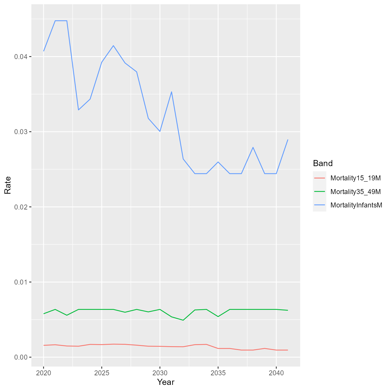
## [97] 0.000 0.000 0.000 0.000 0.000- ratesMatrix : Times-series for banded rates, with stochasticity applied.
library(ggplot2)
library(tidyr)

m <- results[[10]]$PopulationRates$maleMortality$ratesMatrix

df <- data.frame(Year = as.numeric(colnames(m)),
                 MortalityInfantsM = m["MortalityInfantsM",],
                 Mortality15_19M = m["Mortality15_19M",],
                 Mortality35_49M = m["Mortality35_49M",])

dff <- pivot_longer(df, c("MortalityInfantsM", "Mortality15_19M", "Mortality35_49M"),
                    names_to = "Band",
                    values_to = "Rate")

g <- ggplot(data = dff)
g <- g + geom_line(aes(x = Year, y = Rate, group = Band, color = Band))
g